Case Study_OTA (1)

xray4ota ©

• Herein, automated analysis of the trans-conductance amplifier (OTA), universal analog building block, is depicted. The OTA is considered a circuit under test as shown in Figure 3. The outer terminals should be defined as 6x-ports; vin, vip, vdd, vss, vout, and ibiasn wherever, the internal structure of OTA be. Several kinds of analysis are used such as DC, transient, and AC analysis to define district parameters, as listed in tabel 1 and 2.

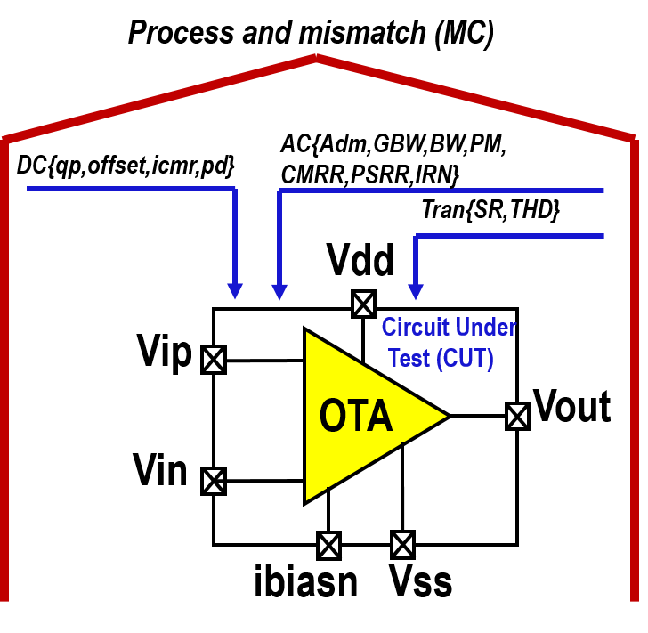
Figure 3. OTA under test.

Table 1 : Analysis vs Paramter

Analysis	Paramter
DC/DC Sweep	Total Current (A)
	Total Power (W)
	Offset (V)
	Vin_min (V)
AC Analysis	Dc-Gain (dB)
	Gain Bandwidth Product (Hz)
	Phase Margin (Deg)
	Bandwidth (Hz)
	CMRR (dB)
	PSRR+ (dB)
	PSRR- (dB)
	Input Referred Noise (V)
Transient Analysis	Slew Rate (V/sec)
	Total Harmonic Distortion (%)

Table 2 : Process and Mismatch Analysis

Analysis	Paramter
Monte-Carlo (MC)	DC-Gain(dB)	Mean (dB)
		Standard Deviation (dB)
		Cabability Process
	Gain Bandwidth Product(Hz)	Mean(Hz)
		Standard Deviation(Hz)
		Cabability Process

The developed tool is utilized to test two different structures of OTA to evaluate the tool’s effectiveness. The used structures of OTA are miller and folded-cascode, as depicted in Figure 4. After using the xray4ota tool, the electrical characteristics of OTAs are listed in the table 3.

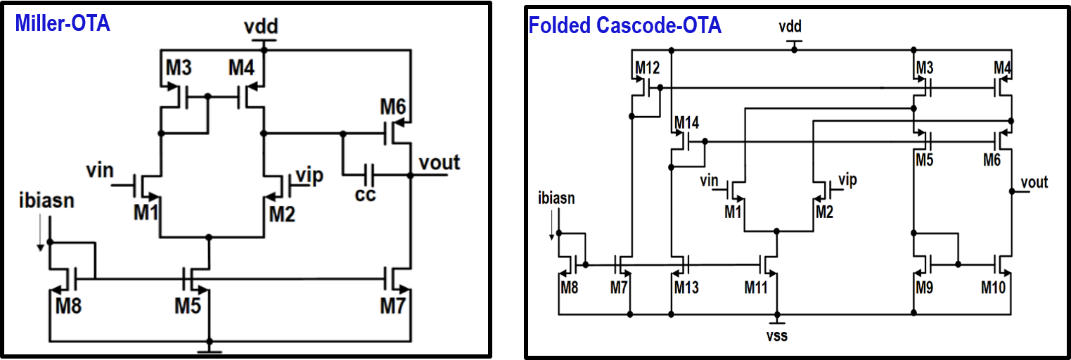
Figure 3. OTA circuit.

Table 3 : Results of xray4ota tool

Analysis	Paramter	Miller Topology	Folded-cascode Topology
DC/DC Sweep	Total Current (A)	0.000176436	7.10188E-05
	Total Power (W)	0.000317585	0.000127834
	Offset (V)	0.0005257	0.0024598
	Vin_min (V)	0.54157	0.547968
AC Analysis	Dc-Gain (dB)	53.6652	43.0194
	Gain Bandwidth Product (Hz)	1.68395E+07	1.58434E+07
	Phase Margin (Deg)	69.1777	76.8771
	Bandwidth (Hz)	34962.6	112787
	CMRR (dB)	65.1424	78.7436
	PSRR+ (dB)	56.21563	73.814
	PSRR- (dB)	53.665	43.019
	Total IRN (V) @ 1MEG	2.29288E-05	2.28478E-05
Transient Analysis	Slew Rate	908993	2.07351E+06
	THD (%)@ Vp of 0.65 V and freq.=1Khz	0.943859	4.85748
Figure of Merits	FOM1=Cl*SR/Pd (f.v/s.w)	2.86e-03	1.62e-02
	FOM2=Cl*GBW/Pd (f.Hz/w)	5.30e-02	1.24e-01

Table 4 : MC results of xray4ota tool

Paramter		Miller Topology	Folded-cascode Topology
DC-Gain (dB)	Mean	27.2	41.2
	Standard Deviation	15.9	5.37
	CP	1.05	3.1
	CPK	0.57	2.56
GBW (Hz)	Mean	7.74e+06	1.57e+07
	Standard Deviation	5.65e+06	8.39e+05
	CP	1.45	9.73
	CPK	0.4	5.84

Usage Steps

xray4ota tool

Please, follow the next steps to guarantee the of usage xray4ota tool effectively.

• Draw the OTA circuit (Folded Cascode, Miller..etc) using XSCHEM, as shownin Figure 4.

• Set all dimensions as design parameters,as shownin Figure 4.

  • Select a device and press “q”.

  • Replace L, W, nf, and mult as listed.

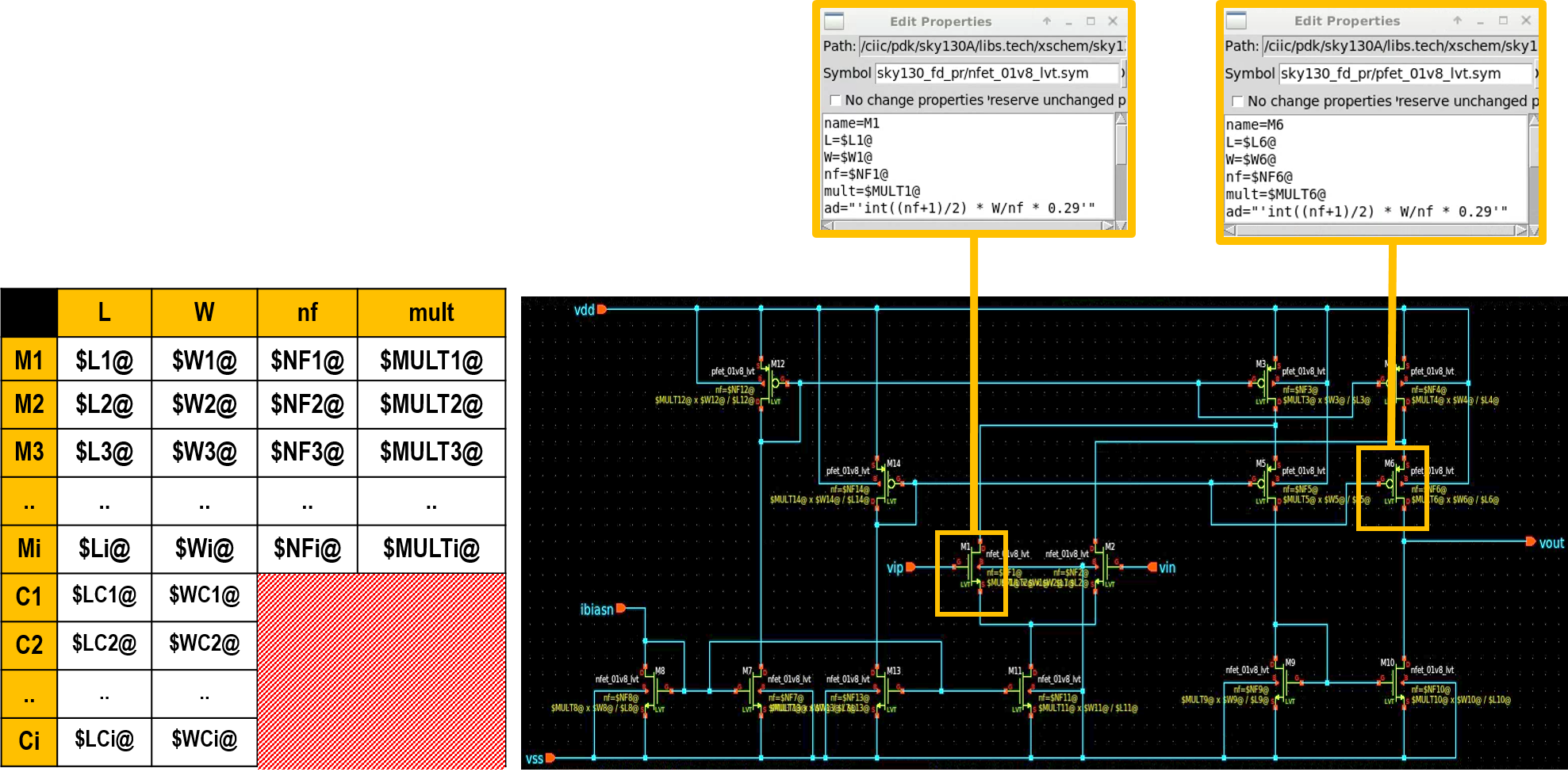
Figure 4. OTA circuit on XSCHEM.

• Make sure the ports’ name as listed in Figure 5.

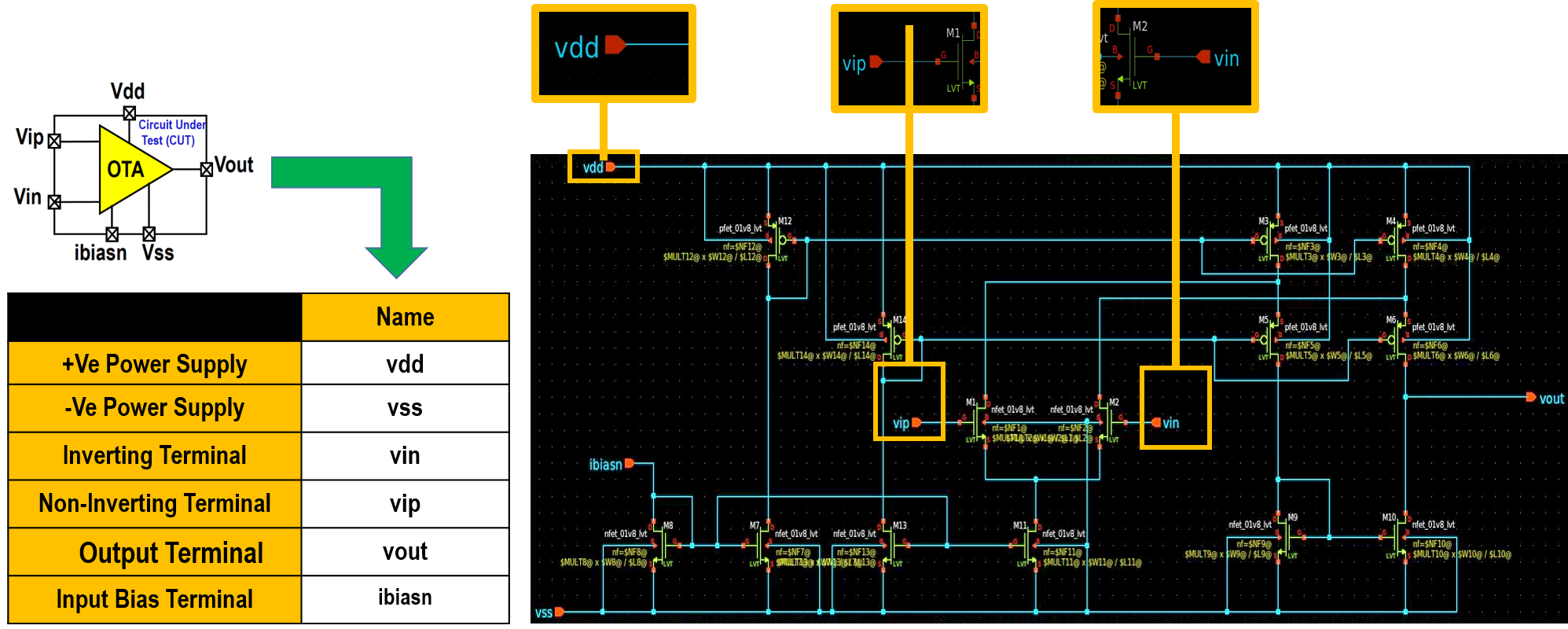
Figure 5. Port name on XSCHEM.

• From XSCHEM as shwon in Figure 6, mark “LVS netlist:Top level is a .subckt”, then press “Netlist”

• Save the netlist as ndiff-ota-circuit.spice

Figure 6. Generate netlist on XSCHEM.

• Open an empty file and save it as a ota.cfg to present a configuration file for the design.

• Open the ota.cfg file and edit the following contents to configure the previous design parameters, as shwon in Figure 7.

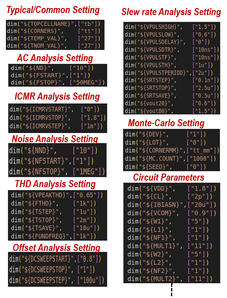
Figure 7. Configuration file

• Open a file and save it as a specifications.txt to present the design specifications.

• Open specifications.txt and edit the following upper/lower specification limits, as shown in Figure 8.

Figure 8. Design specification file

Note

• The designer/user should submit 3X files:

1- ndiff-ota-circuit.spice

2- ota.cfg

3- specifications.txt

• Copy those files to the folder named cut, as shown in Figure 9.

Figure 9. CUT file

• Using the following command in Figure 10, XRAY4OTA script can be executed. Several folders and files are generated, depicted in Figure 11.

Figure 10. Command line

Figure 11. Generated files

• As depicted in Figure 12, checklist lies in summary file.

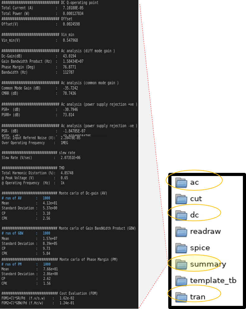
Figure 12. Generated files

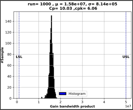
Figure 13. GBW

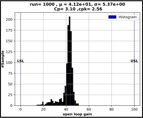
Figure 14. GBW

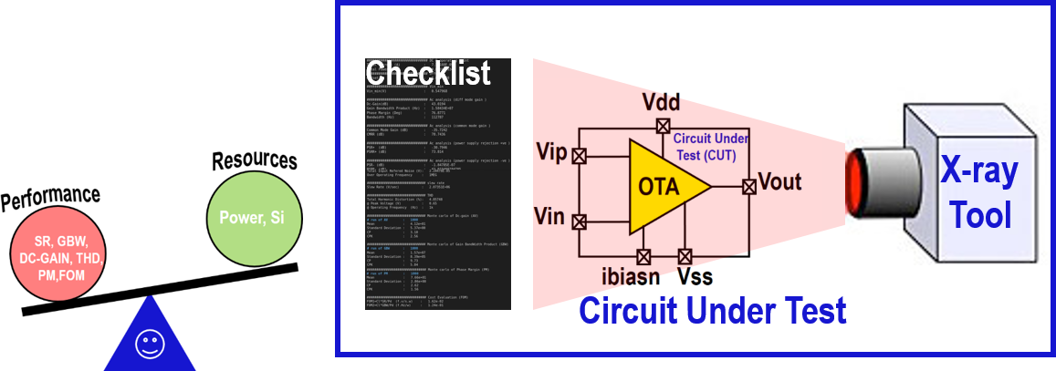
Figure 15. conclsion